We have been looking at the evolution of signalling systems under natural selection. In lecture 3 I motivated this kind of model by talking about alarm calling systems, and briefly mentioning some of the evidence that suggests that alarm calling systems are innate, i.e. independent of experience – that’s already a bit of a simplification, but it’s not a terrible one. Modelling the evolution of innate signalling systems is therefore a sensible place to start, but it’s not going to get us very far in simulating the emergence and evolution of language, because language is learned: you learn the language of your speech community by being exposed to the language they produce. Our next step is therefore to look at learning: we are going to extend our simple model of signalling systems to explore how signalling systems might be learned from experience.
Numerous computational models of learning exist, but one of the best known classes of models are connectionist models, also known as neural network models or artificial neural networks. These models vary in their sophistication and complexity, and you will be relieved to hear that we will be using an extremely simple connectionist model in this course – in fact it’s so simple that proper connectionist modellers would turn up their noses in disgust. But it’s just sophisticated enough for our needs, and it follows on very naturally from the evolutionary models we have been building so far.
What is connectionism?
Although we won’t be using a fancy connectionist model, it will be useful for you to know roughly what a connectionist model is, and how they are used to model learning. Read at least two of the following:
- A very basic introduction to connectionism (everybody should read this, it’s short and simple)
- An introduction to connectionism from a philosophical perspective (read sections 1-5 of this if you want a little more background on connectionism without too many of the modelling details)
- An introduction to connectionism from a modeller’s perspective (read this if you want more details on how connectionist models work)
- A short and fairly dense Scientific American paper on learning in connectionist networks (by one of the legends of the field, for the keen).
What kind of model will we be using?
Hopefully, regardless of which of those tutorials you read, you got the idea that connectionist networks (or neural networks, or artificial neural networks) consist of a set of simple units which are connected to one another. The network learns by adjusting the weights of those connections (perhaps using some kind of error-driven learning, although that’s not what we’ll be doing). And you can retrieve stuff from the network by activating some units and seeing how that activation spreads through the network along the weighted connections. If you didn’t get the gist of that, go back and read another one of the articles I suggested.
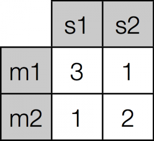
How are we going to model a signalling individual as a neural network? Recall that we are currently modelling individuals as matrices of weights: every individual in our evolution1.py model had a send matrix and a receive matrix, used for sending and receiving. Let’s focus on a send matrix, which looks like this:
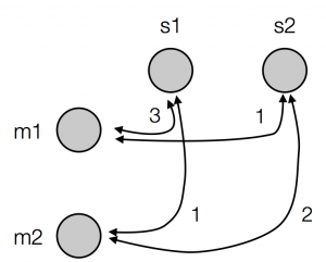
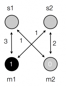
We are using winner-take-all retrieval, so if we want to find out which signal the agent with this production matrix will produce for meaning 1, we look along the row corresponding to m1, find the most strongly-associated signal (in this case, signal 1), and return that. Note that this procedure involves looking at the strengths of association between meanings and signals – if I said “weights” instead of “strengths of association” you could start to see how this matrix is equivalent to a very simple neural network. In fact, instead of drawing our matrix as a matrix, we could draw it as a network, like this:
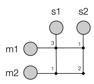
Now the possible meanings are represented as units (circles), all the meanings are connected to all the signals (each connection is a little line), and every connection has a weight (a number next to the line) – but note that the weights on the connections between meanings and signals are the same as the strengths from the matrix above, we are just drawing the same thing in a different way. We could also draw the same matrix as a network like this:
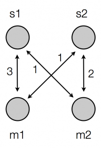
So now the connections are indicated by little diamonds at the intersections of the lines. Or to make it really clear that this is a network just like the networks you saw in the web introductions I linked to above, we could draw it like this:
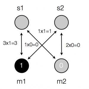
I prefer the middle of those representations, but let’s stick with the last of them for a little while. OK, so now we can write our production matrix down as a simple little neural network. How do we use this network to do production? Well, we activate some units and allow the activation to spread along the weighted connections. So if we want this network to produce a signal for meaning 1, we activate unit m1 (activate means “turn on” – we set its activation to 1) and leave the other meaning unit inactive (its activation is 0).
Then we multiply the activations of the input units by the weights to get the amount of activation that spreads to each of the signal units:
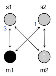
Then we add up the incoming activations at each signal unit:
Finally, we just have to decide which signal unit(s) are going to be activated. Often neural networks use a threshold (i.e. if the total incoming activation is greater than some specific value the unit becomes active, otherwise it doesn’t) or something fancier; instead, we are just going to activate the signal unit with the highest incoming activation, in this case unit s1.
So that’s exactly the same as the winner-take-all process on the matrices – setting activations to 1 or 0 and allowing those activations to spread and then selecting the most active output unit is exactly equivalent to looking along the appropriate row and selecting the signal with the highest strength. If you don’t believe me, come up with a few more examples and verify it for yourself.
And here’s the same process illustrated on the network represented in a way that’s closer to the matrices:
Activation spreading on a network
Learning
The main motivation for thinking about our matrices as networks is that it makes it really obvious how to do learning. In particular, we will start off with an absolutely classic form of learning, Hebbian learning: “any two cells or systems of cells that are repeatedly active at the same time will tend to become `associated’, so that activity in one facilitates activity in the other” (Hebb, 1949). In other words, if we increase connection weights between units that are active, they will tend to become associated in the sense that Hebb identifies – the stronger weight between them makes it more likely that if you activate one unit, the other will be activated.
How are we going to do this in practice? Well, our units represent meanings and signals, and we want to increase the strength of connection between units (meanings and signals) which are active at the same time. Let’s imagine for a moment that learning works like this: a learner hears a signal being produced by some other individual, and perceives the meaning that this signal is intended to convey (maybe the speaker somehow highlights the signal’s meaning for the learner, or maybe the meaning becomes apparent afterwards, or maybe the learner infers it somehow – see discussion below). That means that the learner is observing a pairing of meaning and signal. We’ll call this observational learning: learning through observing the linguistic behaviour of others.
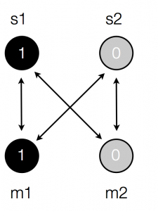
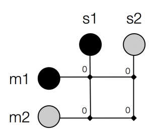
We can represent this by activating the corresponding meaning and signal units. So for instance, if our learner initially has all their weights set to 0, and then observes meaning 1 being conveyed using signal 1, the initial weights and unit activations would look like this:
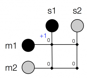
Then, following Hebb’s principle, we strengthen the association between the active units:
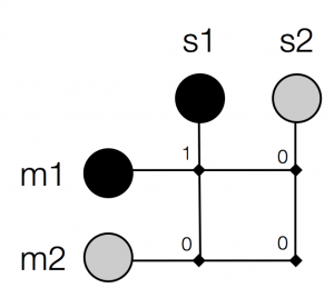
Which gives us a new set of weights:
Or if you prefer to think about this learning process operating on matrices, it would look like this:
Learning illustrated on matrices
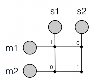
That’s it – that’s all we need to model a learning episode. We can then repeat this process: so say the learner now sees meaning 2 conveyed using signal 2, it ends up with these weights after learning:
And now, thanks to winner-take-all retrieval, meaning 1 and signal 1, meaning 2 and signal 2 have indeed become associated for this learner: activating meaning 1 will tend to lead to production of signal 1, activating meaning 2 will tend to lead to production of signal 2.
That’s it – possibly the simplest model of learning you could hope to find.
Isn’t it weird they the learner observes meanings as well as signals?
A bit, yes! Presumably when you learn words, one of the major challenges you face is to work out what those words mean – you aren’t just handed meanings and signals on a plate, you have to do some inference to work out what the word meaning is (and maybe what the signal is too, if it’s a word contained in a continuous speech stream). At the risk of being dull, I have done some work in this area, and I think the question of how learners infer word meaning is a fascinating one. But it’s not one we’re going to spend much time on in this course: we want a nice simple model of learning, and this is going to be our starting point. If you are worried about it, you could experiment (for example) with a model where the learner infers several possible meanings for each signal (sometimes or often including the correct one), then apply Hebbian learning and see what happens – the results come out roughly the same. Or you could imagine that this model captures what learning is like for socially-adpet individuals like humans, who are good (somehow!) at inferring word meaning. Or you could imagine that the speaker is producing helpful, learner-directed behaviours which make it easy for the learner to infer the word’s meaning. We can also discuss this issue in class if you like.
What now?
That’s it – do the post-reading quiz, look at my comments, then we’ll go over this in class. Come equipped with questions!
References
Hebb, D. O. (1949). The Organization of Behaviour. Wiley: New York, NY.

